Computing Greeks for American Options Part 1

When searching for how to compute the greeks for options, often the Black-Scholes model is brought up. The Black-Scholes model is one of the most popular models and for sure an amazing publication. Still, it does have its drawbacks. One being, that it focuses on European style options, which do not allow early exercise, like American style options do. Since currently the biggest economy in the world is the USA, and the biggest US stock exchanges (NYSE, NASDAQ) provide American style options, these options are an extremely important financial vehicle.

So how do we compute the greeks for those if we should not use the Black-Scholes model? One simple method is the Binomial Options Pricing model. This method is a discrete one in that it builds a tree with nodes at specific discrete times in the lifetime of an option. Note that I will be using Python (numpy) notation below. For instance, let us assume an American call option with the strike price 100$, the underlying stock price being at 100$, the expiration being 6 months to go, and the annualized returns of the stock being defined as:

historical_returns = [1.09, 1.06, 0.90, 0.98, 0.92, 1.06, 0.96, 1.05, 1.09, 1.04, 0.93, 1.1101, 1.08]

Thus, the standard deviation $\sigma{}$ is np.std(historical_returns) = 0.07. Other assumptions include the risk free rate being $1.5\%$ (we use the US Treasury 10y yield at the current point in time). Obviously, the risks of the US defaulting are not 0, but they are hopefully (and likely) extremely small. Lastly, we set a parameter $n$, which sets the depth of the tree and thus the granularity of our calculations. For instance, if the option is $2$ months out but we set $n = 4$, we would compute $4$ discrete values for the $2$ months and segment the $2$ months in $4$ parts (so each segment is $2$ weeks).

The first step in the BOPM is to build the price tree. For this, we need to compute a few helper values:

$u = e^{\sigma{}\sqrt{t}} \\ d = \frac{1}{u}$

where $t$ is the fraction of the year until expiration using Day Count Convention divided by $n$. For example, for 6 months this would be $30 * \frac{6}{360} = \frac{1}{2} = 0.5$. $u$ is the implied volatility upwards and $d$ is simply the reverse (so downwards).

We simply go through each segment of the $6$ months in our example (so from $n=1$ to $n=4$) and compute the upward and downward movement from the last point. The next upwards price would be $P * u$. The resulting tree looks like this:

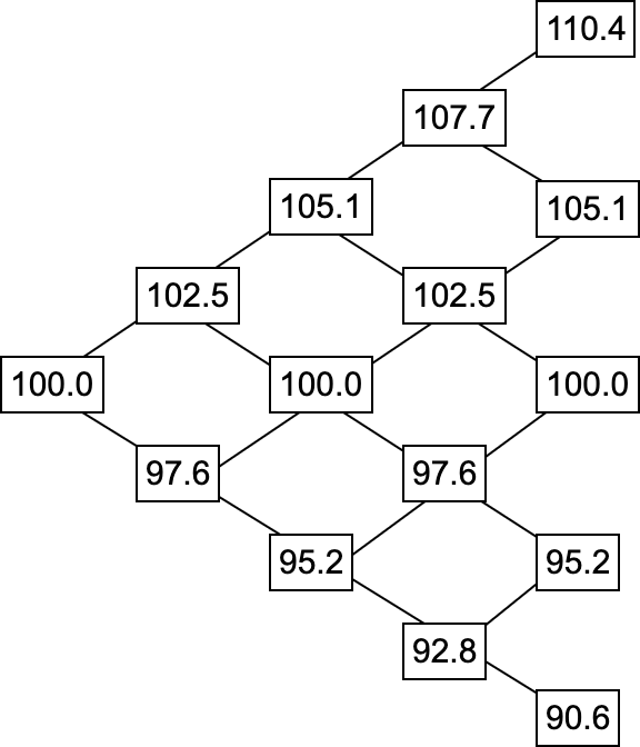
Note that in our example, $u = e^{0.07\sqrt{\frac{0.5}{4}}} = 1.025$ and $d = \frac{1}{1.025} = 0.976$. Starting at $100$, the first upward move is $100 * 1.025 = 102.5$ and the first downward move is $100 * 0.976 = 97.6$. The upward from $102.5$ on would be $102.5 * 1.025 = 105.1$, and so on.

The second step is computing the value at expiration for each possible option value. This is actually rather simple: Take the last price for each scenario (so for each leaf node of the tree on the very right) and subtract the strike price from it. Specifically, one has to compute max(last_price - strike_price, 0). Note that this is for calls - for puts one needs to compute max(strike_price - last_price, 0). This already enables European options, but American options are still open.

The third step is computing all the intermediary option values at different time steps, which enables American options. Since this is a bit more involved, this is left open for part 2!